A lot of attention has been spent on attention mechanisms, where they come from, connections to prior techniques (like kernel methods), and so on, and rightfully so. Attention layers have been instrumental in the biggest AI revolution we've seen in our lifetime: the large language model. Comparatively, the successful exemplars and applications for convolutional nets consist of the generative latent diffusion models used in image generation and processing. It's not to say that people don't talk about convolutional nets, but it is to say that people maybe talk a little more about the motivation behind attention mechanisms. It may be because convolutional nets are somewhat easier to motivate, starting from kernels for edge detection or similar convolutional features and then generalizing to arbitrary kernels is not a hard sell. Despite that, convolutions are really, really elegant formally and have quite satisfying ways of being seen.
What is a convolution? Is it a product like \((f * g)(x) = \int_{\mathbb{R}^n} f(y)g(x-y) \ dy\)? Well, that's one way of looking at a convolution. To me however the definitive way to think about convolutions would be as linear, translation invariant, continuous maps (of appropriate functions). Translation invariance is really the key idea here. In specific terms, translation commutes with convolution in the following sense: with \(\tau_h\phi (t) = \phi(t - h)\) denoting translation by \(h\) as an action on a function we have
\begin{equation} \begin{aligned} u * (\tau_h \phi) &= \\ \int_{\mathbb{R}^n} u(y)\phi(x - y - h) \ dy &= \\ \int_{\mathbb{R}^n} u(y)\phi([x-h] - y) \ dy &= \\ \tau_h(u * \phi). \end{aligned} \end{equation}That's pretty trivial or straightforward to see, just commutativity, associativity of addition. What is interesting however is the following: if any linear map on (suitably regular and 'nice') functions which happens to be continuous (in the appropriate sense) is also translation invariant, then it is given as a convolution against a distribution (or generalized function) [1]. I apologize for all of the 'suitably' and 'appropriate sense,' but the specific definitions would make the article more mathematically loaded and not for much gain. There's no real devil hiding in those hypotheses, this is just really a defining characteristic of translation invariant regular maps.
There are two big connections here I'd like to cover. First is the connection to differential equations. The defining characteristic of constant coefficient differential operators is their translation invariance in the same way. When you look at a finite difference for approximating a derivative (an expression like \(\Delta_h f(x) = \frac{f(x+h) - f(x-h)}{2h}\), which numerically approximates the derivative for small \(h\)) like the numerical Laplacian used in edge detection, it is a convolution against a kernel which is, for example, \(-1\) to the first area to the left of \(0\) and \(1\) to the first area to the right of \(0\) and \(0\) at \(0\) itself and \(0\) elsewhere. Basically, it looks like a staircase: \(-1\), \(0\), \(1\). We can think of this from the convolutional perspective from first principles, without knowing what a finite difference operator "should" look like beforehand. We have:
\begin{equation} \int_{\mathbb{R}^n} u(y) \phi(x-y) \ dy = \phi'(x) \end{equation}and we have:
\begin{equation} \begin{aligned} \phi'(x) &= \\ \int_{\mathbb{R}^n} \delta(y - x) \phi'(x) \ dy &= \\ \int_{\mathbb{R}^n} \delta(y) \phi'(x - y) \ dy &= \\ -\int_{\mathbb{R}^n} \phi(x-y) \frac{d}{dy}[\lim_{\alpha \rightarrow 0} \frac{e^{-(y/\alpha)^2}}{|\alpha| \sqrt{\pi}}] \ dy \end{aligned} \end{equation}where we used integration by parts and the assumption that \(\phi\) is nonzero only on a bounded area in \(\mathbb{R}^n\) (compact support) to ensure the disappearance of any boundary terms (since differentiation is local we could replace \(\phi\) by a function identical to it on a small area around \(x\) anyway if need be to obtain a similar expansion). We used the limit \(\delta(y) = \lim_{\alpha\rightarrow 0} \frac{e^{(y/\alpha)^2}}{|\alpha| \sqrt{\pi}}\), representing the Dirac-δ as a limit of Gaussian bell curves with \(0\) variance. We can figure out that the finite difference operator would look like it does from the fact that the bell curve with near \(0\) variance looks like a big positive spike (similar to another approximate δ function) at the left inflection point and symmetrically a negative spike at the right inflection point and an odd (as in antisymmetric, an odd function) curve from the left inflection point to the right (for a more rigorous derivation: use the trapezoidal rule and some approximations that work for small \(\alpha\)), so we should expect to see it picking out the left neighbor value negatively, taking nothing near the center (due to the odd integrand there), and then picking out the right hand value positively. If you work through the approximation more rigorously, you'll recover the finite difference expression. I included a picture of the derivative as a visual aid. The conclusion is just that convolutions reproduce a lot of different useful operators because a lot of different useful operators are translation invariant, which probably occurs so much because the laws of nature are invariant with respect to space and a mean-value approximation often suffices for variations in many quantities. I think that also emphasizes the limitation of convolutions in and of themselves though.
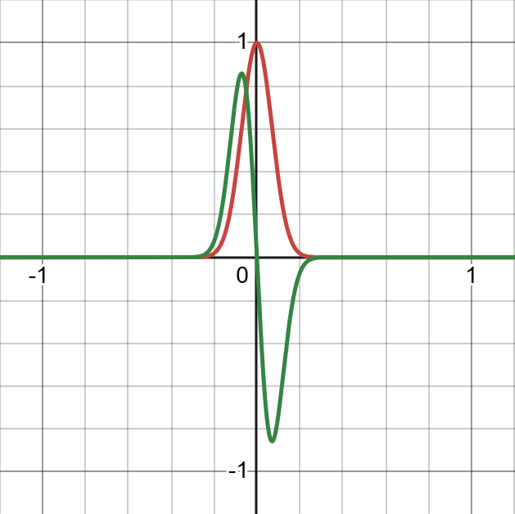
A Gaussian with its Derivative
On either side of zero, the derivative looks like it approximates Dirac delta distributions, near zero the contributions cancel eachother out. The convolution against the derivative as the variance goes to zero behaves like the derivative of the function being convolved against evaluated at 0.
Okay, so what about the second connection? Well, it's a little niche, but essentially you can view a convolution as the result of forcefully making something invariant under a family of transformations. Suppose we have a binary function like \(f(x, y) : \mathbb{R}^2 \rightarrow \mathbb{R}\) and we want to make it commutative. You can of course just define: \(g(x, y) = \frac{f(x, y) + f(y, x)}{2}\), the average of the two results. A convolution is a sum over the images of translations like: \(u(0)\phi(x) \rightarrow u(y) [\phi(x-y)]\). If you remember from probability theory, a convolution calculates the P.D.F. for the sum of two R.V.s, by summing over all the substitutions which don't affect the sum of the arguments of the two factors in the integrand: \(0 + x = y + (x-y)\). In that way a convolution only cares about the substitution to the extent it changes the sum of the integrands (hence it only commutes with translations, rather than being entirely invariant under them). The reasoning there is a little sloppy, I'll write more about it some day I think, but maybe you get the gist of what I mean. In general you can look for transformations which are invariant under or commute with some symmetry and I think we should really focus a lot more on that in learning. We already kind of do it, for example "Alias-Free Generative Adversarial Networks" [2] studies 'equivariance' (we'd call it "commutativity") of operations with respect to translation and rotation in the "analog" domain (of a recovered signal a la Nyquist-Shannon sampling) for a convolutional image-generation net: we should get the same results if we translate, rotate the continuous representation (recovered from the discrete samples) as if we rotate, translate, and then recover the continuous form. That's a form of anti-aliasing, since it involves showing that our operations respect the Nyquist frequency and don't generate too-high frequency content. Still, one thing I've never seen is "weak" commutativity, e.g. losses that reward similarity or punish divergence from a commutative law. For example, a pitch shifting network could have a loss term which encourages translation along a latent dimension to commute with translation of pitch in the dataset (e.g. translating by \(1\) in the latent dim gives the same result as translating by a semitone in the input data and keeping all else equal), using cosine similarity, losses on the difference, or similar. I think a good stochastic weak loss for this kind of thing would be interesting to see and could serve as a great way to integrate inductive biases in a weak enough way to avoid reducing model flexibility. When you think about it "weak" commutativity actually covers a rather massive swathe of inductive biases we have.
Anyway, that's about it. I think convolutions are still interesting, more as a prototype for symmetry based layers, and obviously they will always be useful because translation invariance will always be relevant because it is a part of our natural world. There's a lot more to write about convolutions too.
References
[1] Lars Hormander, The Analysis of Linear Partial Differential Operators I, Second Edition, pp. 100-101
[1] note: I can't find a damn date of publication for the publication run of this book I want to cite, and thankfully I'm not writing a formal article so I don't have to. Apparently it was republished by Springer in 2003, the Springer copyright in my copy is dated 1990, the foreword was written in 1989, so a fair estimate is that it probably got out around 1990. Everyone who ever writes a \(\partial\) should read this book. Even if you don't find linear PDE interesting, it is one of the most compelling expositions of any mathematical topic I have ever read.
[2] Alias-Free Generative Adversarial Networks, Karras et al., 2021, 35th Conference on NeurIPS
[2] note: this is a decent article, but the legacy of this technique is a little complicated. At the end of the day all of the 'equivariance' talk boils down to conditions on the frequencies generated when assuming a fixed bandwith for our inputs (as per the Nyquist-Shannon sampling theorem/scheme), so the prescription is just low pass filtering. The only other paper I've seen to use these ideas would be BigVGAN's anti-aliased periodic activation functions, where anti-aliasing is supposed to help smooth out artifacts in the generated audio and in the spectrograms. So it isn't a great example of commutativity being used in practice even if it is theoretically exactly like that, because the case it uses is a quite classical and simple one to the extent that the basic prescription is just an LPF rather than e.g. any kind of loss. Also I have heard mixed results about the technique itself in practice, later works would not wind up utilizing its contributions consistently. Make of that what you will.