attention

Convolutions are translation invariant: they produce features which depend on nearby values in the input data in a linear, spatialy homogeneous way, meaning the value of a specific filter at $y_i$ is a linear function of nearby values $x_j, i-n \leq j \leq i+n$, but the filter can't change as we move over the sequence. Since this function is a linear map $w : \mathbb{R}^{2n+1} \rightarrow \mathbb{R}$, it can be represented by a $1 \times (2n+1)$ matrix $w_{ij}$ relative to the standard basis: a row vector, where the matrix multiplication representing the linear action $wv$ is given by a dot product against $w_{1j}$. Translation invariance just means that this vector, which is the kernel of the convolution, is the same for every $y_i$. This is useful because it approximately describes many natural operators very well and it means you only need to keep track of the kernel and a bias, rather than the massive size a dense layer would have. Differentiation does not care where you are, it only cares what nearby values look like, and it is linear, so it may be represented as a convolution (against $-\delta'(x)$: you can get a more interesting representation by using a sequence of smooth functions approximating $\delta(x)$ trying to differentiate under the limit sign). The solution to any linear PDE with constant coefficients is also easily treatable in terms of convolutions as well for similar reasons, and constant coefficient approximations for PDEs with spatially varying coefficients can work in some cases, so people will often opt for a constant coefficient approximation if they expect e.g. the heat-conducting properties of a material to be roughly homogeneous. So for any kind of spatial, physical signal, convolutions, despite their simplicity, actually are very expressive. As an additional large caveat the kernels in ML are finite and usually small (small-kernels). That means that many convolutional operations like inverting differential operators should be off the table (they are non local operators: the values of their outputs at a point depend on values far away, usually globally i.e. they depend on values everywhere). However in practice finite approximations can work pretty well especially in a situation where you are grossly overparameterizing the function you are trying to approximate, so even if we can't apply the Poisson kernel exactly, we could get something very close in two or three layers, and especially close insofar as we particularly care about. But regardless of how large we can get our receptive field, convolutions will always be translation invariant. They are not well suited to modeling spatially inhomogeneous relationships where we care a great lot about something happening in a far away place more than we care about something happening nearby. Let's say there's an important piece of data that every part of the output should care about. You'd need a kernel large enough to 1. find the area of interest, 2. take on sufficiently large values near that area of interest to amplify it. But unless that piece of data is disproportionately large compared to the nearby data, then if we move three steps to the right in our output data, we'll care just as much about the nearby data three steps to the right of the "important-piece" in the input as we did about the important piece before we took three steps to the right in our output. Consider the figure below.

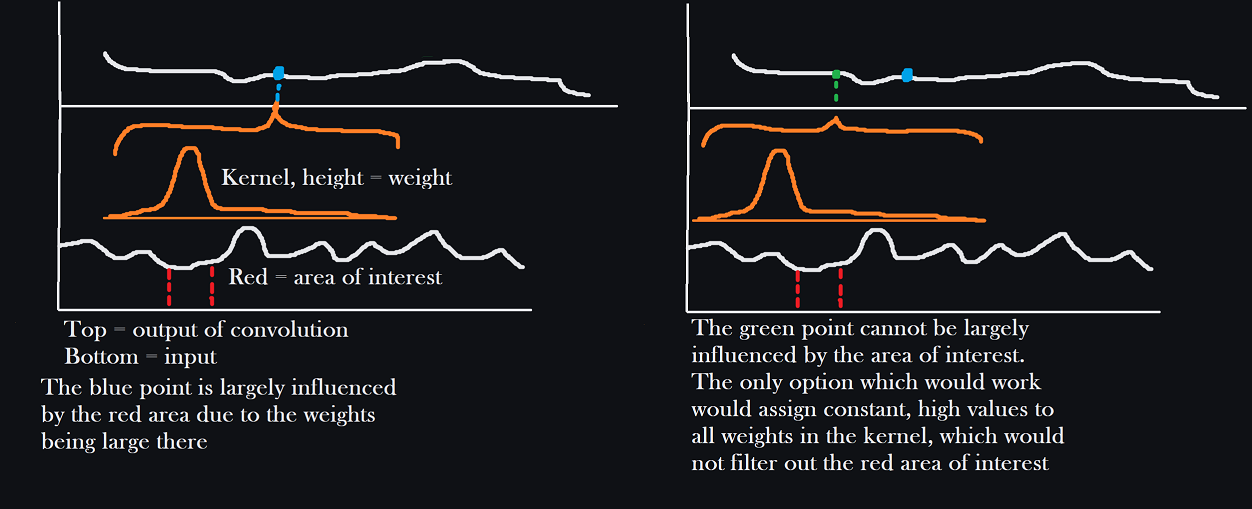
However natural language is quite a different beast where we do not have similar reason to believe that operations which are 'like' applying the heat operator to a function, or applying the heat kernel, etc, would be inherently useful. No matter what we do with convolutions, they're always going to average up nearby data for points in the output. We'd like to make things less localized in that way and connect things based on specific information arbitrarily. We are still dealing with, for the sake of the discussion and in most applications, a sequence-to-sequence problem, but the outputs can depend on inputs all over the place, without the kind of uniformity you get form a convolution. We often have just the issue seen in the figure then, where we want many output things to be influenced by many input things in arbitrary places as the data dictates. We really want something like a multiplexer: we have a bunch of signals, representing notable features in the input sequence (which can come from anywhere).

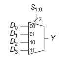
A multiplexer takes a control signal and a bunch of inputs and outputs only one of the outputs one of its inputs based on the specific value of the control signal. If for every day of the week a different person in your $7$ person friend group gets to decide where to eat, it's kind of like what we want and kind of like a multiplexer. You each have your own preference, which is the information about the sequence we're inspecting at a given point, but based on the day of the week (the control signal) only one of you will have an effect on the output.

Let the signal representing information around the item at position $i$ be $h_i$. This could be as simple as $x_i$, the exact value at that position, or anything else we decide on later, like an average of values nearby, or whatever it is. The point is it is one of many potential signals we are interested in routing to some area we're doing computation, like figuring out what to emit for a single token in an autoregressive model. The next big thing we need to decide on is representing our control signal. The control signal is going to tell us which of the $h_i$ we want to focus on. If we're working emitting a value at position $j$ we'll write $a(h_i, C_j)$ to represent how important the information near input element $i$ is as per some context $C_j$, which could for instance be, a token we are emitting,

It seems at this point then reasonable to choose the largest $h_i$ with the largest $a(h_i, C_j)$ as the most important thing to focus on, or as the output for the multiplexer. The main issue with a straightforward maximum is that it impairs gradient flow. Okay, what if we used a softmax? We average the $h_i$ with the weights as dictated by a softmax. If you want to calculate the actual maximum in a vector of items using $\operatorname{argmax}$ (the one softmax is an approximation for, the one that returns a vector with $1$ in the spot where the maximum item in the input vector was and $0$ elsewhere), it looks like $\langle operatorname{argmax}(v), v \rangle$. Since softmax is an approximation for argmax, we can replace argmax with it. Let's put our signals into vector form: $\mathbf{h}_i = h_i$, and $\mathbf{a}_i = a(h_i, C_j)$. We want to pick the element of $\mathbf{h}$ for which the corresponding 'importance' $\mathbf{a}_i$ is largest. If we did an argmax over $\mathbf{a}$, then we would just take the dot product again but this time against $\mathbf{h}$, to pick out only that value. In symbols:

$$\textit{most relevant input} = \langle\operatorname{softmax}(\mathbf{a}), \mathbf{h}\rangle = \Sigma \alpha_i h_i$$

where:

$$\alpha_i = \operatorname{softmax}(\mathbf{a})_i = \frac{\exp(a_i)}{\Sigma^k \exp(a_k)}.$$

You can think of the entire thing as producing a multinomial distribution over the local data $h_i$ using softmax and then taking the expectation, which isn't too dissimilar from softmax-multinomial, the use of softmax layers to emit multinomial distributions in classification problems. In that way, you can see the whole 'multiplexer' thing we've discussed here as a small network to classify which input signal ($h_i$, in this case representing local data in some area of the whole input sequence) is relevant to the output we're processing right now. All that's left is to specify structures for $h_i$ and $a$. We want to of course use linear maps for everything.

We decide to keep it simple: we want $\mathbf{h}$ to be the same length as $\mathbf{x}$, the input sequence, and we can project the vector at $x_i$ down into something smaller. The choice of projection is like focusing on looking for specific types of inputs or specific words, specific semantic clusters. That makes it easy to implement, we just have linear map (a linear layer) we learn to take each vector in the input sequence down to a lower-dimensional subspace: $h_i = Kx_i$. Ok, what about $a(h_i, C_j)$? We ultimately want a single number to come from this representing the importance of $h_i$ to the computation with context $C_j$, so the obvious choice is to to use a linear map to make the two of the same dimension and then take the dot product: $a(h_i, C_j) = \langle h_i, Q C_j \rangle = x_i^TK^T Q C_j$, which is the usual expression you see in attention formulations.

Now we don't have to write $h_i = Kx_i$. We could simply write $h_i = x_i$ and then put $K^T$ inside of the calculation for $a$. That's particularly convenient if we want to model the sequence itself end to end. In that case, the whole output of our little multiplexer at $j$:

$$\Sigma x_i \frac{\exp(a_i)}{\Sigma^k \exp(a_k)} = \Sigma x_i \frac{\exp(x_k^TK^T Q C_j)}{\Sigma^k \exp(x_k^TK^T Q C_j)}.$$

Basically all it takes at this point is choosing to set $C_j = x_j$ to get "self-attention." I'll come back to all of this later and expand, since attention is an interesting topic. But maybe you can get the motivation for attention that way. The choice of linear maps is obvious and the desire to create something like a multiplexer also is.