convolution

I have written a lot on convolutions. Most are familiar with the basic idea already. I will include a few pieces of my writing on convolutions as I find them relevant here. In short, I find the canonical point of view regarding convolutions to be that they are uniquely the translation invariant linear maps on functions of suitable kinds. TODO: add pseudocode for every type of convolution common in ML (causal, with many filters, boundary conds).

Translation Invariant Linear Maps

A foreword from fully-convolutional:

Convnets are built on translation invariance. Their basic components (convolution, pooling, and activation functions) operate on local input regions, and depend only on relative spatial coordinates.

What is a convolution? Is it a product like $(f * g)(x) = \int_{\mathbb{R}^n} f(y)g(x-y) \ dy$? Well, that's one way of looking at a convolution. To me however the definitive way to think about convolutions would be as linear, translation invariant, continuous maps (of appropriate functions). Translation invariance is really the key idea here. In specific terms, translation commutes with convolution in the following sense: with $\tau_h\phi (t) = \phi(t - h)$ denoting translation by $h$ as an action on a function we have

$$ \begin{aligned} u * (\tau_h \phi) &= \ \int_{\mathbb{R}^n} u(y)\phi(x - y - h) \ dy &= \ \int_{\mathbb{R}^n} u(y)\phi([x-h] - y) \ dy &= \ \tau_h(u * \phi). \end{aligned} $$

That's pretty trivial or straightforward to see, just commutativity, associativity of addition. What is interesting however is the following: if any linear map on (suitably regular and 'nice') functions which happens to be continuous (in the appropriate sense) is also translation invariant, then it is given as a convolution against a distribution (or generalized function) [1]. I apologize for all of the 'suitably' and 'appropriate sense,' but the specific definitions would make the article more mathematically loaded and not for much gain. There's no real devil hiding in those hypotheses, this is just really a defining characteristic of translation invariant regular maps.

There are two big connections here I'd like to cover. First is the connection to differential equations. The defining characteristic of constant coefficient differential operators is their translation invariance in the same way. When you look at a finite difference for approximating a derivative (an expression like $\Delta_h f(x) = \frac{f(x+h) - f(x-h)}{2h}$, which numerically approximates the derivative for small $h$) like the numerical Laplacian used in edge detection, it is a convolution against a kernel which is, for example, $-1$ to the first area to the left of $0$ and $1$ to the first area to the right of $0$ and $0$ at $0$ itself and $0$ elsewhere. Basically, it looks like a staircase: $-1$, $0$, $1$. We can think of this from the convolutional perspective from first principles, without knowing what a finite difference operator "should" look like beforehand. We have:

$$ \int_{\mathbb{R}^n} u(y) \phi(x-y) \ dy = \phi'(x) $$

and we have:

$$ \begin{aligned} \phi'(x) &= \ \int_{\mathbb{R}^n} \delta(y - x) \phi'(x) \ dy &= \ \int_{\mathbb{R}^n} \delta(y) \phi'(x - y) \ dy &= \ -\int_{\mathbb{R}^n} \phi(x-y) \frac{d}{dy}[\lim_{\alpha \rightarrow 0} \frac{e^{-(y/\alpha)^2}}{|\alpha| \sqrt{\pi}}] \ dy \end{aligned} $$

where we used integration by parts and the assumption that $\phi$ is nonzero only on a bounded area in $\mathbb{R}^n$ (compact support) to ensure the disappearance of any boundary terms (since differentiation is local we could replace $\phi$ by a function identical to it on a small area around $x$ anyway if need be to obtain a similar expansion). We used the limit $\delta(y) = \lim_{\alpha\rightarrow 0} \frac{e^{(y/\alpha)^2}}{|\alpha| \sqrt{\pi}}$, representing the Dirac-\delta as a limit of Gaussian bell curves with $0$ variance. We can figure out that the finite difference operator would look like it does from the fact that the bell curve with near $0$ variance looks like a big positive spike (similar to another approximate \delta function) at the left inflection point and symmetrically a negative spike at the right inflection point and an odd (as in antisymmetric, an odd function) curve from the left inflection point to the right (for a more rigorous derivation: use the trapezoidal rule and some approximations that work for small $\alpha$), so we should expect to see it picking out the left neighbor value negatively, taking nothing near the center (due to the odd integrand there), and then picking out the right hand value positively. If you work through the approximation more rigorously, you'll recover the finite difference expression. I included a picture of the derivative as a visual aid. The conclusion is just that convolutions reproduce a lot of different useful operators because a lot of different useful operators are translation invariant, which probably occurs so much because the laws of nature are invariant with respect to space and a mean-value approximation often suffices for variations in many quantities. I think that also emphasizes the limitation of convolutions in and of themselves though.

Markov Chain Connection

A one-dimensional convolutional layer with total kernel size $k$ assumes that the output at token $n$ comes from a linear functional (a mapping that takes a vector and yields a scalar, which in coordinates is just a dot product) applied to $k$-vector of values prior or nearby values (potentially dilated). In terms of how it's conditioning, it looks like a Markov chain on a $k$-gram: $f(x_n, ..., x_1) = f(x_n | x_{n-1}, ... x_{n-k})$. That last part also equals $f(x_{n+m} | x_{n+m-1}, ... x_{n+m-k})$ [note that this last equality should be interpreted as a functional equality: if the $k$-grams we are conditioning on are the same, then the densities for each potential value of $x_n$ and $x_{n+m}$ are the same] where the last equality is representing the fact that we have one kernel for the whole convolution, so the probability only depends on the packet of values in the $k$-gram and does not vary based on where we are in the sequence. This property is known as "translation invariance," but if you're looking at things from the Markov chain analogy point of view you could just say that it's expressing the fact that the Markov dynamics are not magically changing throughout 'time' or in different places. Markov chains can be seen as stochastic generalizations of finite state machines or systems of ODEs that give dynamics for dynamical systems: in the second interpretation, the order of the $k$-grams being processed is analogous to the number of equations in the the system of ODEs being considered once all equations have been put in first order (using the trick where we write $y' = u$ and then substitute $u'$ for $y''$ everywhere), or for single equations, it's analogous to the order of the ODE, which is perhaps more intuitive since you need initial conditions of equal number to initialize either for similar reasons. The point being that in this analogy the time-invariance (or the property of being autonomous) of the dynamics of physical systems for example (e.g. $-\nabla U(x) = mx''$ which does not depend on $t$ explicitly) is analogous to the translation invariance or being stationary of a Markov chain. So no matter what it just comes down to this algebraic "translation invariance" idea.

The canonical point of view here is 'translation invariance' (which maybe should be called translation commutativity, but it's quite common to call commutativity laws of this kind 'invariance' laws): we have for all $g_h(t) = g(t-h)$ the following identity $(f * g_h)(t) = (f * g)(t-h)$. In other words, if we translate one of our inputs first, then it's the same as translating the resulting convolution in the same way. We can interchange the order of translation and convolution (hence 'translation commutativity,' translation commutes as an operator on functions with convolution). You can also put the 'time invariance' of a dynamical system in a more direct way. For a system of ODEs, the system ultimately looks like $\frac{dx}{dt} = f(t, x(t))$ (in general, a vector equation) and of course for an autonomous system we have $\frac{df}{dt} = 0$.

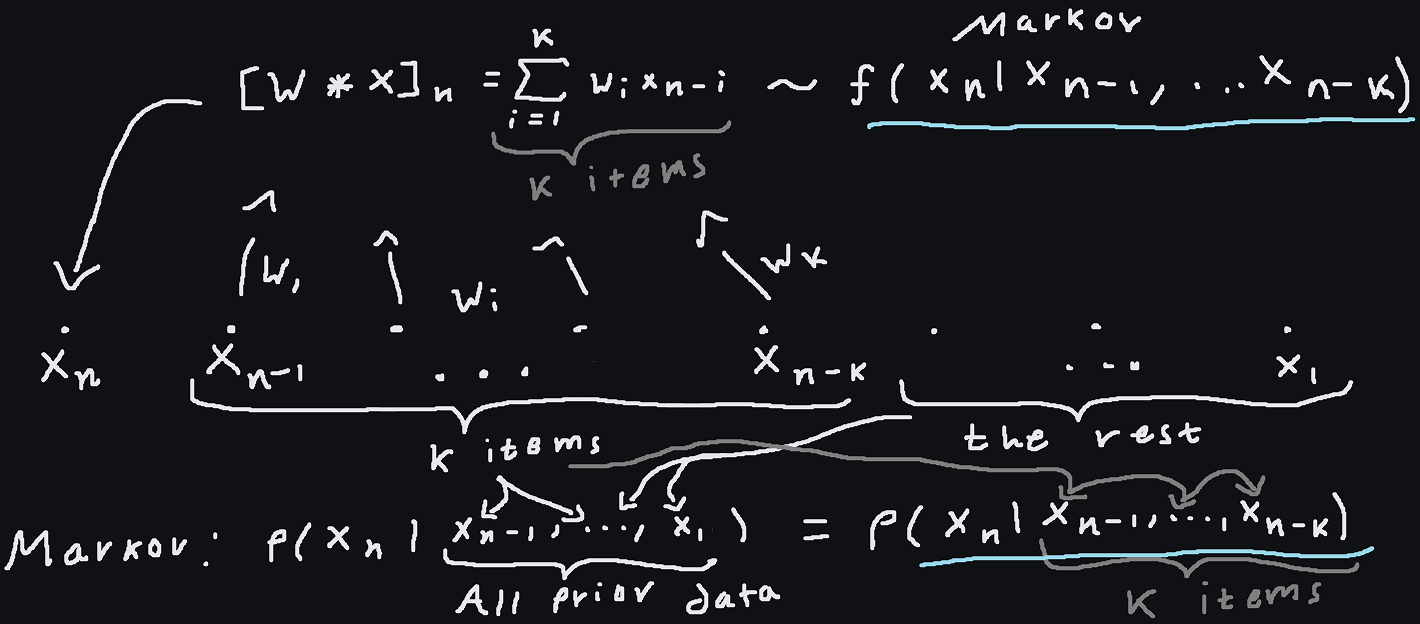
In the sketch, we see a brief summary of the relationship graphically. A convolution is essentially a linear, translation invariant transformation (LTI, does that ring a bell anyone? Yes, such systems in engineering are easy to treat with generalized functions precisely because they are so readily modeled by and reasoned about by convolutions) and has the proper 'dependencies' or conditions $x_n$ on the correct quantities (the prior $k$ values of $x$). It's notable however that the convolution yields a deterministic model for the result, rather than prescribing a stochastic model. In PixelRNN, the RNN approach conditions similarly to the CNN approach (both starting with an autoregressive decomposition), but with no finite-time limit and no simple time invariance. Actually, every time invariant linear transformation can be expressed as a convolution if it operates in a suitably regular way on suitably regular functions [1], so convolutions (of sufficiently wide kernel sizes) can represent any such transformation.

• References

[1] Lars Hormander, The Analysis of Linear Partial Differential Operators I, Second Edition, pp. 100-101