Pixel Recurrent Neural Networks

'Pixel Recurrent Neural Networks' by Van den Oord et al: https://arxiv.org/pdf/1601.06759. I'm not going to lie to you and say that this paper would be profound by today's standards. However I think it is a very illustrative example of a story you're probably going to get used to seeing a lot of times. To start with, this paper is centered on RNNs and the motivation is basically just autoregression. Autoregression was desirable because it makes modeling joint distributions a little more straightforward and computationally tractable. You write $f(x,y,z) \rightarrow f(x)f(y | x)f(z | x, y)$ and then you try to stuff all the conditional logic into an RNN (in this case) whose state carries information useful for generating the next token assuming you've seen all the prior ones. In this paper, the autoregression happens from the top left corner to the bottom right, in writing order like we in the west would write on a piece of paper (decidedly not a case of the meme idiotropy) In comparison a one-dimensional convolutional layer with total kernel size $k$ assumes that the output at token $n$ comes from a linear functional (a mapping that takes a vector and yields a scalar, which in coordinates is just a dot product) applied to $k$-vector of values prior or nearby values (potentially dilated). In terms of how it's conditioning, it looks like a Markov chain on a $k$-gram: $f(x_n, ..., x_1) = f(x_n | x_{n-1}, ... x_{n-k})$ [A]. This 'finite memory' or 'Markov' property of convolutions connects below to an important theme, the notion of a 'receptive-field', where a convnet has a finite 'receptive-field' because it's ultimately a stack of conditional probabilities that each only depend on nearby values in a finite range.

What is a receptive-field? For a convolution, it is what the kernel sees at a given point, like laying the kernel over the point in question and marking the pixels covered. In more general terms though (e.g. for an RNN), how far away can an input pixel be while influencing the output at a given pixel? For RNNs, hypothetically this is quite adaptive and dependent on the state transitions. For a CNN, it's bounded above due to a simple theorem on the supports of convolutions, or alternatively, just looking at a graph of the connections. It goes up multiplicatively in the kernel sizes. So convolutional nets have a fixed receptive-field size. To put it in obvious terms the value at $f * g (n) = \Sigma_{-k/2 \leq m \leq k/2} f(m - n)g(m)$ for example (assuming $k$ is even) depends on $k$ values of $f$ around $n$. I want to reiterate that a thorough-going theme here in my document and opinion is that the useful heuristics for choosing models tend to be their hypothetical capacity to connect input features to output features, something like 'feature-connectivity.' In the case of images like this, receptive-fields encode that: the wider a receptive-field, the more we can connect input features far away from a given output pixel to its value. All of this makes sense because the features for inputs and outputs are the same for images. In general when that's the case looking at the capacity of a network to abstractly connect information in relevant places (e.g. graphically if it suits your intuition) is a recurrent theme.

The first RNN structure described is the 'Row-LSTM' model, which is a hybrid convolution-LSTM model. The structure is like so: we run a convolution over an entire row and then we run an LSTM over each row of input-to-state features like a vector, going down the image. A word is in order about causal convolutions. Causal convolutions involved masking or shifting the data so that a convolution doesn't use data e.g. ahead of the current index being computed in a sequential processing task. So of course these convolutions have to be causal, like any convolutions for autoregressive tasks. The primary relevance is that since we are generating from top left to bottom right, and during generation we could look at the pixel to our left, but with our convolutions running row-wise, such a thing is not in the cards for our input-state calculations. An innovation in this paper (for its time) is the use of diagonal BiLSTM to alleviate this issue, where the LSTM processes one diagonal at a time (both forwards and backwards, hence bi) rather than proceeding along the axes of the image. The use of a skewed (diagonal) window of attention allows for full utilization of already-generated data. This idio-syncratic sort of direction is a meme I call idiotropy in analogy with isotropy, anisotropy, orthotropy. The diagonal model performed best in this paper unsurprisingly. Although on an individual level the change in receptive-field may seem minor, the information propagates throughout the network, meaning that the diagonal model actually sees quite a lot more than the row model.

A few other memes appear in this paper. A multi-scale model is developed, which essentially does a full run of the network on a subsampled version of the image for multiple levels of subsampling, and then conditioning each less subsampled layer on the output of the prior one, which is an example of hierarchical processing. Another important and recurring meme is the (further..) discretization of output variables. A multinomial model is used a la softmax-multinomial to represent the output RGB values as taking values in a discrete range. This meme often presents itself in conjunction with autoregression, although the association is not necessary (which is sometimes stated). For example, in this paper, a continuous model was tried, but found to be less performant. Discretization is often a logical and elementary technique to employ when floating-point representations are too fine-grained. A subtle meme is small-kernels, which we can see evidenced in: "Besides reaching the full dependency field, the Diagonal BiLSTM has the additional advantage that it uses a convolutional kernel of size 2x1 that processes a minimal amount of information at each step yielding a highly non-linear computation. Kernel sizes larger than 2x1 are not particularly useful as they do not broaden the already global receptive field of the Diagonal BiLSTM." However a larger kernel is used during the first layer when the autoregressive masking is first applied. I'll still mark this as small-kernels since the convnet only has 3x3 kernels past that point. The use of relu activations in the convolutional version of PixelRNN is present, as is usual for all recurrent nets at this time.

Footenote [A]

That last part also equals $f(x_{n+m} | x_{n+m-1}, ... x_{n+m-k})$ [note that this last equality should be interpreted as a functional equality: if the $k$-grams we are conditioning on are the same, then the densities for each potential value of $x_n$ and $x_{n+m}$ are the same] where the last equality is representing the fact that we have one kernel for the whole convolution, so the probability only depends on the packet of values in the $k$-gram and does not vary based on where we are in the sequence. This property is known as "translation invariance," but if you're looking at things from the Markov chain analogy point of view you could just say that it's expressing the fact that the Markov dynamics are not magically changing throughout 'time' or in different places. Markov chains can be seen as stochastic generalizations of finite state machines or systems of ODEs that give dynamics for dynamical systems: in the second interpretation, the order of the $k$-grams being processed is analogous to the number of equations in the the system of ODEs being considered once all equations have been put in first order (using the trick where we write $y' = u$ and then substitute $u'$ for $y''$ everywhere), or for single equations, it's analogous to the order of the ODE, which is perhaps more intuitive since you need initial conditions of equal number to initialize either for similar reasons. The point being that in this analogy the time-invariance (or the property of being autonomous) of the dynamics of physical systems for example (e.g. $-\nabla U(x) = mx''$ which does not depend on $t$ explicitly) is analogous to the translation invariance or being stationary of a Markov chain. So no matter what it just comes down to this algebraic "translation invariance" idea.

The canonical point of view here is 'translation invariance' (which maybe should be called translation commutativity, but it's quite common to call commutativity laws of this kind 'invariance' laws): we have for all $g_h(t) = g(t-h)$ the following identity $(f * g_h)(t) = (f * g)(t-h)$. In other words, if we translate one of our inputs first, then it's the same as translating the resulting convolution in the same way. We can interchange the order of translation and convolution (hence 'translation commutativity,' translation commutes as an operator on functions with convolution). You can also put the 'time invariance' of a dynamical system in a more direct way. For a system of ODEs, the system ultimately looks like $\frac{dx}{dt} = f(t, x(t))$ (in general, a vector equation) and of course for an autonomous system we have $\frac{df}{dt} = 0$.

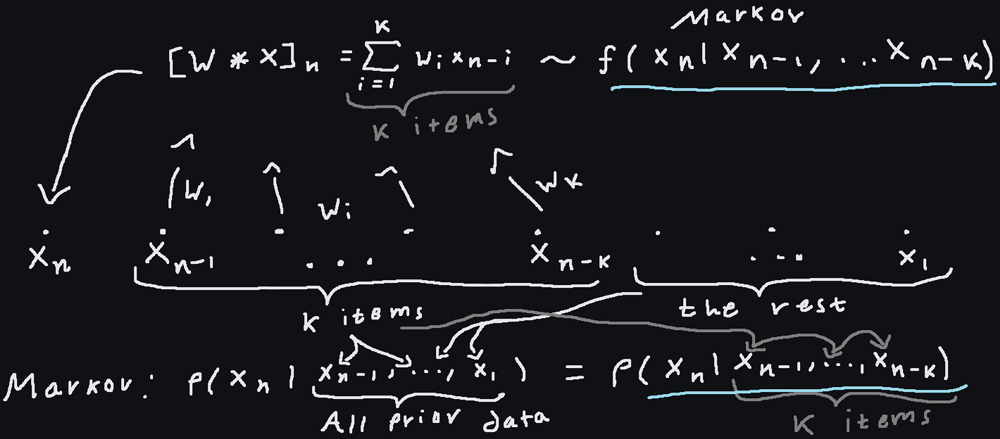
In the sketch, we see a brief summary of the relationship graphically. A convolution is essentially a linear, translation invariant transformation (LTI, does that ring a bell anyone? Yes, such systems in engineering are easy to treat with generalized functions precisely because they are so readily modeled by and reasoned about by convolutions) and has the proper 'dependencies' or conditions $x_n$ on the correct quantities (the prior $k$ values of $x$). It's notable however that the convolution yields a deterministic model for the result, rather than prescribing a stochastic model. In PixelRNN, the RNN approach conditions similarly to the CNN approach (both starting with an autoregressive decomposition), but with no finite-time limit and no simple time invariance. Actually, every time invariant linear transformation can be expressed as a convolution if it operates in a suitably regular way on suitably regular functions [1], so convolutions (of sufficiently wide kernel sizes) can represent any such transformation.

Like most 'finite-memory' type circumstances (e.g. on FSM versus full Turing machines or PDA), what counts as 'state' or 'memory' is quite liberal. In our case it takes on a rather concrete meaning, but for example, we could form a tagged union of all the possible subsequences of observations and call the observed state at moment $n$ to be the full sequence of observations from $x_1$ to $x_{n-1}$ so that $x_n$ can depend on the entire sequence as though it had arbitrary memory, but it is nothing more than rephrasing the autoregressive decomposition to do so.