Unet

"U-Net: Convolutional Networks for Biomedical Image Segmentation," Ronneberger et al., https://arxiv.org/pdf/1505.04597. This model is a descendant of alexnet, a sibling to vggnet. Important themes in this paper are training-data and inductive-bias. The elephant in the room however is the unet structure, which mixes ushape with unet-skips. Despite being named after Unet, the network architecture is almost entirely derived from fcnet. By ushape, I mean that the model reduces the dimensions of its input until it reaches a critical point in the middle, often called the bottleneck, although distinct from small bottleneck layers as seen in resnet, before again raising dimension in a symmetric manner. The point of the ushape structure in Unet here is spatial: the downsampling operations are maxpool 2x2 operations which give coarser and coarser views of the input data at different spatial resolutions, allowing the network access to a hierarchical stack of abstractions, each containing data on a different scale of locality. The successive downsampling is akin to taking lower and lower resolution views of an image, hence encoding information about the signal more spread out in adjacent pixels after each downsample. Since Unet happens to use small-kernels (an independent 'mutation' seemingly not derived from vggnet) (correction! This meme was inherited from fcnet through vggnet!), downsampling and depth are the only ways to attain a larger receptive field. A downsample followed by a convolution is essentially equivalent to a dilated-convolution, which wavenet used instead of downsampling. In the authors' own words:

The main idea in [9] is to supplement a usual contracting network by successive layers, where pooling operators are replaced by upsampling operators. Hence, these layers increase the resolution of the output. In order to localize, high resolution features from the contracting path are combined with the upsampled output. A successive convolution layer can then learn to assemble a more precise output based on this information.

A visual overview of the specific architecture can be seen here (taken from the paper, p. 2):

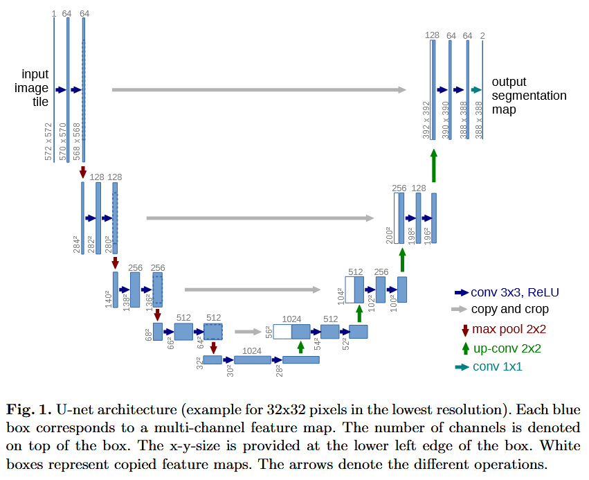
The second relevant meme for Unet to mention here is obvious: the horizontal connections running parallel to the downsampling operations. These are unet-skips, and they connect by concatenation the representations on the left hand side to the corresponding representations on the right hand side, pairing representations which are of the same level of spatial locality. In this case the representations would be of similar dimension if it were not due to the loss of pixels on the borders, since this Unet implementation did not pad to preserve spatial dimensions. Therefore the left-hand-side representations are cropped prior to concatenation. Then on the righthand side transposed-convolutions are used to upsample the data spatially. A transposed convolution is in linear algebraic terms the transpose of a strided convolution as a linear map [A]. One less 'formal' way to think of a transposed convolution is that instead of laying a kernel onto the tensor/image and taking the inner product (the sum of products formed with the kernel value at each point with the tensor's value at that point), you multiply the kernel in a transposed convolution by the value of the tensor at a point, and then lay the kernel out onto the area around that point in the tensor. The complexity enters the picture when strides are introduced, but it is also, really, the main point of a transposed convolution. A normal convolution with stride $2$ cuts the shape of its input in half (with proper padding). A transposed convolution has to do the opposite. When you go from one point to the next in a transposed convolution with stride $2$, the kernel is no longer laying over the exact same spot as in the original tensor. Now the way it works is like this: suppose we have a flat rectangular grid representing an image. We make a copy of the grid and scale it up by a factor of $2$, but we keep the coordinate axes the same. Then the transposed convolution at each point multiplies the kernel by the value on the original grid there, but places it in the corresponding spot on the stretched grid, effectively adding twice as many new elements by spacing the kernels apart by two units each in the output, hence doubling the length and width of the resulting grid. I have included a picture from "A guide to convolution arithmetic for deep learning," Dumoulin and Visin, https://arxiv.org/pdf/1603.07285. The footnote contains more details albeit in more mathematical language.

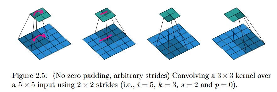
The point of all this is to say that the transposed convolutions are used to increase the spatial resolution so we can symmetrically scale back up. This is a very common technique, but Unets helped to popularize this sort of thing (even if fully-convolutional seemingly 'introduced' it to the literature). Another point of view to consider with transposed-convolutions is that of a stride smaller than $1$ in a normal convolution, where the kernel moves less than one unit, producing many more entries in the resulting tensor:

Another way to connect coarse outputs to dense pixels is interpolation. For instance, simple bilinear interpolation computes each output $y_ij$ from the nearest four inputs by a linear map that depends only on the relative positions of the input and output cells. In a sense, upsampling with factor $f$ is convolution with a fractional input stride of $1/f$. So long as $f$ is integral, a natural way to upsample is therefore backwards convolution (sometimes called deconvolution) with an output stride of $f$. Such an operation is trivial to implement, since it simply reverses the forward and backward passes of convolution.

from fully-convolutional, p. 4. I will probably add more regarding Unet later, since it is such a critical network.

Footnote on Transpose Convolutions

The transpose may always be calculated from a matrix representation in the usual way, but it also may be calculated by solving $\langle u, K_s * v \rangle = \langle K_s^T u, v \rangle$ for $K_s^T$, where $K_s$ is a convolution with stride $s$ and where $\langle , \rangle$ is the inner product, which for discrete sequences or finite sequences (regular vectors) is the dot product, and which for functions over a common domain is $\langle f, g \rangle = \int f(x)g(x) \ dx$. Naturally $K_s * v$ is a downsampled tensor (in the most general sense, because it halves the size of the support), and $u$ must be of the same shape. In order for the equality to hold $K_s^T u$ needs to upsample $u$. If $v = \delta(x - x_0)$ then we get:

$$(K_s^T u)(x_0) = \langle u, K_s * \delta(x-x_0) \rangle$$

so that if we can evaluate the term on the right we'll have an expression for the transpose of $u$. Now

$$K_s * \delta(x-x_0) (y) = \int k(sy - x)\delta(x-x_0) \ dx = k(sy - x_0)$$

so we have:

$$(K_s^T u)(x_0) = \langle u(y), k(sy - x_0) \rangle = \int u(y) k(sy - x_0) \ dy. $$

Setting $u = \delta(y-y_0)$ we get:

$$(K_s^T \delta(y-y_0))(x_0) = \langle delta(y-y_0), k(sy - x_0) \rangle = k(sy_0 - x_0), $$

where for tensors the $\delta$ functions are just the standard coordinate functions. Where a normal transpose has the coordinate representation:

$$(K_s \delta(x-x_0))(y_0) = \langle \delta(x-x_0), k(sy_0 - x) \rangle = k(sy_0 - x_0),$$

from which we can see that the only difference is swapping the order of the indices $x_0$ and $y_0$. Let's suppose our functions/tensors are one dimensional and $k$ is $0$ outside of $[-m, m]$. As a function of $y_0$, $k(sy_0 - x_0)$ is $0$ outside of $[-m/s, m/s]$ even at $x_0 = 0$, whereas for $x_0$ it retains its normal character. The columns in the matrix point of view for $K_s^T$ are translates of $k$ run 'backwards:' $C_{ij} = k(sy_i - x_j)$, and as an operator acting on functions that only take on nonzero values in a bounded area like $[-N, N]$, we can assume $C_{ij} = 0$ when $j > N$. When $|i| > 2N/s$, we have $C_{ij} = 0$ for all $j$.